
The following article is an excerpt (Chapter 3) from the book Hands-On Big Data Modeling by James Lee, Tao Wei, and Suresh Kumar Mukhiya published by our friends over at Packt. The article addresses the concept of big data, its sources, and its types. In addition to this, the article focuses on giving a theoretical foundation about data modeling and data management. Readers will be getting their hands dirty with setting up a platform where we can utilize big data.
Digital systems are progressively intertwined with real-world activities. As a consequence, multitudes of data are recorded and reported by information systems. During the last 50 years, the growth in information systems and their capabilities to capture, curate, store, share, transfer, analyze, and visualize data has increased exponentially. Besides these incredible technological advances, people and organizations depend more and more on computerized devices and information sources on the internet. The IDC Digital Universe Study in May 2010 illustrates the spectacular growth of data. This study estimated that the amount of digital information (on personal computers, digital cameras, servers, sensors) stored exceeds 1 zettabyte, and predicted that the digital universe would to grow to 35 zettabytes in 2010. The IDC study characterizes 35 zettabytes as a stack of DVDs reaching halfway to Mars. This is what we refer to as the data explosion.
Most of the data stored in the digital universe is very unstructured, and organizations are facing challenges to capture, curate, and analyze it. One of the most challenging tasks for today’s organizations is to extract information and value from data stored in their information systems. This data, which is highly complex and too voluminous to be handled by a traditional DBMS, is called big data.
Defining Data Models
This article walks the reader through various structures of data. The main types of structures are structured, semi-structured, and unstructured data. We will also be applying modeling techniques to these types of data sets. In addition, readers will learn about various operations on the data model and various data model constraints. Moreover, the article gives a brief introduction to a unified approach to data modeling and data management.
Data Model Structures
Data models deal with data variety characteristics of the big data. Data models describe the characteristics of the data. There are two main sources of data:
- Structured data
- Unstructured data
Structured Data
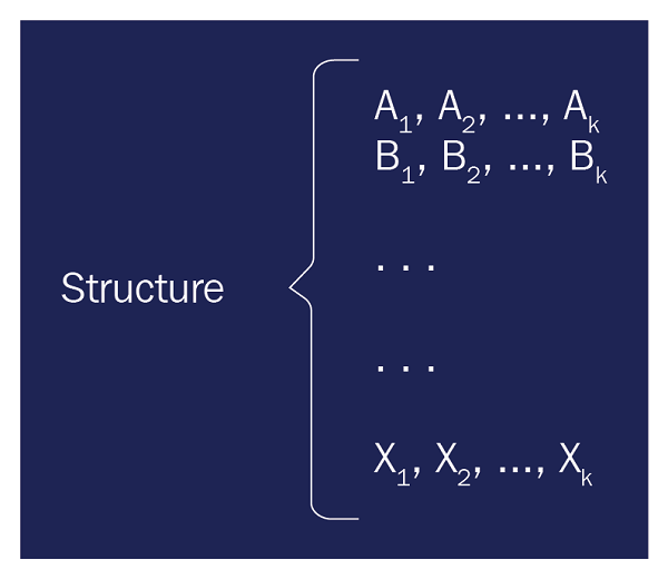
Structured data relates to data that has a defined length and format. Some common examples of structured data include numbers, dates, and groups of words and numbers, which are called strings. In general, structured data follows a pattern like that in Figure 3.1. Generally, the data has predefined columns and rows. Some of the data columns could be missing, but they are still classified as structured data:
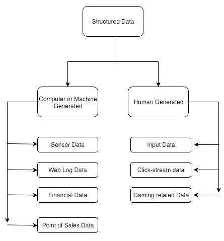
As shown in Figure 3.2, most of the structured data set can be categorized into either computer-generated or human-generated data. Computer-generated structured data includes sensors data, web log data, financial data, and point-of-sales data. Human-generated data includes social media activities and events:
Sensor data sets are generated by sensors. Some of them include radio-frequency ID tags, smart meters, medical devices, smartwatch sensors, and Global Positioning System (GPS) data. The following snippet shows a Comma-Separated Value (CSV) example of sensor data, which includes position identifier, trip identifier, latitude, longitude, and timestamps:
“pos_id”,”trip_id”,”latitude”,”longitude”,”altitude”,”timestamp””1″,”3″,”4703.7815″,”1527.4713″,”359.9″,”2017-01-19 16:19:04.742113″”2″,”3″,”4703.7815″,”1527.4714″,”359.9″,”2017-01-19 16:19:05.741890″”3″,”3″,”4703.7816″,”1527.4716″,”360.3″,”2017-01-19 16:19:06.738842″”4″,”3″,”4703.7814″,”1527.4718″,”360.5″,”2017-01-19 16:19:07.744001″”5″,”3″,”4703.7814″,”1527.4720″,”360.8″,”2017-01-19 16:19:08.746266″”6″,”3″,”4703.7813″,”1527.4723″,”361.3″,”2017-01-19 16:19:09.742153″”7″,”3″,”4703.7812″,”1527.4724″,”361.8″,”2017-01-19 16:19:10.751257″”8″,”3″,”4703.7812″,”1527.4726″,”362.2″,”2017-01-19 16:19:11.753595″”9″,”3″,”4703.7816″,”1527.4732″,”362.9″,”2017-01-19 16:19:12.751208″”10″,”3″,”4703.7818″,”1527.4736″,”363.9″,”2017-01-19 16:19:13.741670″”11″,”3″,”4703.7817″,”1527.4737″,”364.6″,”2017-01-19 16:19:14.740717″”12″,”3″,”4703.7817″,”1527.4738″,”365.2″,”2017-01-19 16:19:15.739440″”13″,”3″,”4703.7817″,”1527.4739″,”365.4″,”2017-01-19 16:19:16.743568″”14″,”3″,”4703.7818″,”1527.4741″,”365.7″,”2017-01-19 16:19:17.743619″”15″,”3″,”4703.7819″,”1527.4741″,”365.9″,”2017-01-19 16:19:18.744670″”16″,”3″,”4703.7819″,”1527.4741″,”366.2″,”2017-01-19 16:19:19.745262″”17″,”3″,”4703.7819″,”1527.4740″,”366.3″,”2017-01-19 16:19:20.747088″”18″,”3″,”4703.7819″,”1527.4739″,”366.3″,”2017-01-19 16:19:21.745070″”19″,”3″,”4703.7819″,”1527.4740″,”366.3″,”2017-01-19 16:19:22.752267″”20″,”3″,”4703.7820″,”1527.4740″,”366.3″,”2017-01-19 16:19:23.752970″”21″,”3″,”4703.7820″,”1527.4741″,”366.3″,”2017-01-19 16:19:24.753518″”22″,”3″,”4703.7820″,”1527.4739″,”366.2″,”2017-01-19 16:19:25.745795″”23″,”3″,”4703.7819″,”1527.4737″,”366.1″,”2017-01-19 16:19:26.746165″”24″,”3″,”4703.7818″,”1527.4735″,”366.0″,”2017-01-19 16:19:27.744291″”25″,”3″,”4703.7818″,”1527.4734″,”365.8″,”2017-01-19 16:19:28.745326″”26″,”3″,”4703.7818″,”1527.4733″,”365.7″,”2017-01-19 16:19:29.744088″”27″,”3″,”4703.7817″,”1527.4732″,”365.6″,”2017-01-19 16:19:30.743613″”28″,”3″,”4703.7819″,”1527.4735″,”365.6″,”2017-01-19 16:19:31.750983″”29″,”3″,”4703.7822″,”1527.4739″,”365.6″,”2017-01-19 16:19:32.750368″”30″,”3″,”4703.7824″,”1527.4741″,”365.6″,”2017-01-19 16:19:33.762958″”31″,”3″,”4703.7825″,”1527.4743″,”365.7″,”2017-01-19 16:19:34.756349″”32″,”3″,”4703.7826″,”1527.4746″,”365.8″,”2017-01-19 16:19:35.754711″…………………………………………………………..
Code block: 3.1 Example of GPS sensors data where columns represent position identifier, trip identifier, latitude, longitude, altitude, and timestamps, respectively.
Structured human-generated data can be input data, click-stream data, or gaming-related data. Input data can be any piece of data that a human might feed into a computer, such as a name, phone, age, email address, income, physical addresses, or non-free-form survey responses. This data can be helpful for understanding basic customer behavior.
Click-stream data can generate a lot of data when users navigate through websites. This data can be recorded and then used to analyze and determine customer behavior and buying patterns. This data can be utilized to learn how a user behaves on the website, discover the process followed by the user on the website, and find out a flaw in the process.
Gaming-related data includes activities of the users while they are playing games. Every year, more and more people are using the internet to play games on a variety of platforms, including computers and consoles. Users browse on the web, send emails, chat, and stream high-definition video.
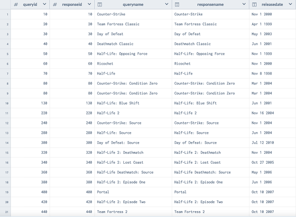
This data can be helpful in learning how end users go through a gaming portfolio. Figure 3.3 shows an example of how gaming-related data looks:
Structured is a regulated format for presenting information about a page and classifying the page’s content. These datasets are of finite length and in a regular format. One of the real usages of a structured dataset is how Google uses structured data that it finds on the web to understand the content of the page, as well as to gather information about the web and the world in general. For example, here is a JSON-LD structured snippet that might appear on the contact page of the Unlimited Ball Bearings corporation, describing their contact information:
<script type=”application/ld+json”>{ “@context”: “http://schema.org“, “@type”: “Organization”, “url”: “http://www.example.com“, “name”: “Unlimited Ball Bearings Corp.”, “contactPoint”: { “@type”: “ContactPoint”, “telephone”: “+1-401-555-1212”, “contactType”: “Customer service” }}</script>
Unstructured Data
Any documents, including clinical documentation, personal emails, progress notes, and business reports, that are composed primarily of unstructured text with little or no predefined structure or metadata describing the content of the document can be classified as unstructured data. Unstructured data is different from structured data in the sense that its structure is unpredictable.
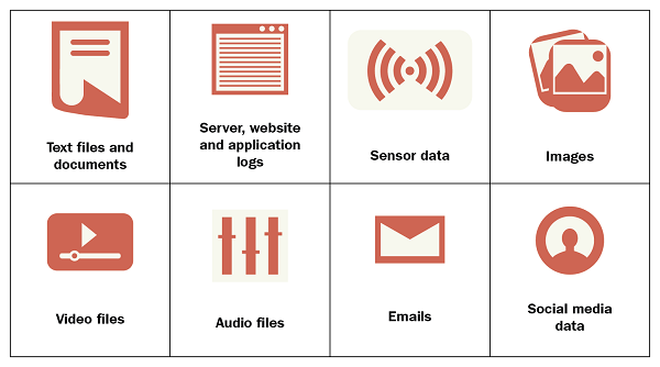
Examples of unstructured data include documents, emails, blogs, reports, minutes, notes, digital images, videos, and satellite imagery. It also incorporates some data produced by machines or sensors. In fact, unstructured data accounts for the majority of the data that’s on any company’s premises, as well as external to any company in online private and public sources, such as LinkedIn, Twitter, Snapchat, Instagram, Dribble, YouTube, and Facebook.
Sometimes, metadata tags are attached to give information and context about the content of the data. The data with meta information is referred to as semi-structured. The line between unstructured and semi-structured data is not absolute, though some data-management consultants dispute that all data, even the unstructured kind, has some degree of structure:
Sources of Unstructured Data
Unstructured data can be located everywhere. In fact, most individuals and organizations operate and store unstructured data throughout their entire life. Unstructured can be either machine-generated or human-generated. Most of the machine-generated unstructured data is satellite images, scientific data, photographs, or radar data:
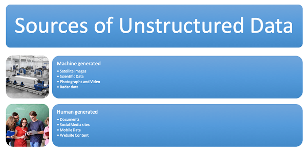
As shown in the preceding diagram, unstructured data can also be classified as machine-generated or human-generated. Most of the machine-generated data sets are satellite images, scientific data, photographs and videos, or radar or sonar data. Most of the human-generated unstructured data sets are documents, social media data, mobile data, and website contents.
Comparing Structured and Unstructured Data
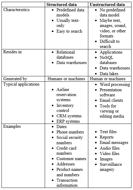
Let’s compare structured and unstructured data with respect to its characteristics, storage, generation, and types of applications where it can be found:
Data Operations
The second component of a data model is a set of operations that can be performed on the data. In this module, we’ll discuss the operations without considering the bigness aspect. Now, operations specify the methods to manipulate the data. Since different data models are typically associated with different structures, the operations on them will be different. But some types of operations are usually performed across all data models. We’ll describe a few of them here. One common operation extracts a part of a collection based on the condition.
Subsetting
Often, when we’re working with a huge dataset, we will only be involved in a small portion of it for your particular analysis. So, how do we sort through all the extraneous variables and observations and extract only those we need? This process is introduced to as subsetting:
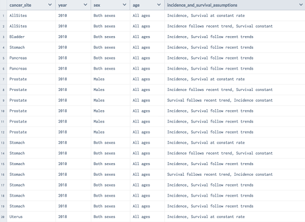
In the example shown in Figure 3.7, we have a set of records in which we are looking for a subset that satisfied the condition and the cancer is for both sexes. Depending upon the context, it is also called selection or filtering. If we need to render the list of records where cancer is seen in both male and female, we can do the following:

Union
The assumption behind the union operation is that the two collections involved have the same structure. In other words, if one collection has four fields and another has 14 fields, or if one has four fields on people and their date of birth, and the other has four fields about countries and their capitals, they cannot be combined through a union.
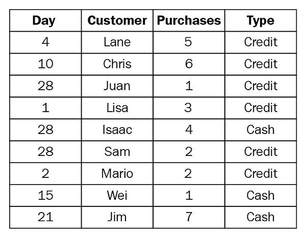
For example, suppose you have the following customer purchase information stored in three tables, separated by month. The table names are May 2016, June 2016, and July 2016. A union of these tables creates the following single table that contains all rows from all tables:

If we perform the union operation on these three tables, we get a combined table:
Projection
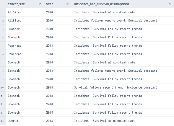
Another common operation is retrieving a specified part of a structure. In this case, we specify that we are interested in just the first three fields of a collection of records. But this produces a new collection of records that has only these fields.
This operation, like before, has many names. The most common name is projection:
Join
The second kind of combining, called a join, can be done when the two collections have different data content but have some common elements. Let’s imagine we have two different tables and they hold information about the same employees. This is the first table that holds identifying information, such as first name, last name, and date:
| 101 | John | Smith | 10-12-2018 |
| 102 | Suresh Kumar | Mukhiya | 10-13-2018 |
| 103 | Anju | Mukhiya | 10-14-2018 |
| 104 | Dibya | Davison | 10-15-2018 |
This is the second table, which holds additional information about the same employee. The table contains three fields: identifier, department, and salary:
| 101 | Information System | $70000 |
| 102 | Account | $50000 |
| 103 | Engineering | $100000 |
| 104 | Human Resources | $788090 |
Joining these two tables should produce a third table with combined data. It also helps to eliminate duplicates:
| 101 | John | Smith | 10-12-2018 | Information System | $70000 |
| 102 | Suresh Kumar | Mukhiya | 10-13-2018 | Account | $50000 |
| 103 | Anju | Mukhiya | 10-14-2018 | Engineering | $100000 |
| 104 | Dibya | Davison | 10-15-2018 | Human Resources | $788090 |
Data Constraints
Besides the data model structure, data model operations, and data model constraint, is the third component of a data model. Constraints are the logical statements that must hold for the data. There are different types of constraints. Different data models have different ways to express constraints.
Types of Constraints
There are different types of constraints:
- Value constraints
- Uniqueness constraints
- Cardinality constraints
- Type constraints
- Domain constraints
- Structural constraints
Value Constraints
A value constraint is a logical statement about data values. For example, say the value of the entity (for example, age) cannot be negative.
Uniqueness Constraints
This is one of the most important constraints. This constraint benefits us by uniquely identifying each row in the table. For example, most of the website doesn’t allow multiple accounts for the same person. This can be enforced by uniqueness constraints. For instance, by making email unique. It is possible to have more than one unique column in a table.
Cardinality Constraints
It’s easy to see that enforcing these constraints requires us to count the number of titles and then verify that it’s one. Now one can generalize this to count the number of values associated with each object and check whether it lies between an upper and lower bound. This is referred to as the cardinality constraint.
Type Constraints
A different kind of value constraint can be enforced by restricting the type of data allowed in a field. If we do not have such a constraint, we can put any type of data in the field. For example, you can have -99 as the value of the last name of a person—of course, that would be wrong. To ensure this does not happen, we can enforce the type of the last name to be a non-numeric alphabetic string. The preceding example shows a logical expression for this constraint.
A type constraint is a special kind of domain constraint. The domain of a data property or attribute is the possible set of values that are allowed for that attribute. For example, the possible values for the day part of the date field can be between 1 and 31, while a month may have the value between 1 and 12, or a value from the set January, February till December.
Domain Constraints
Domain constraints are user-defined data types, and we can define them like this:
Domain Constraint = data type + Constraints (NOT NULL / UNIQUE / PRIMARY KEY / FOREIGN KEY / CHECK / DEFAULT).
For example:
- Possible day value could be between 1-31
- Possible month value could be between January, February till December
- Grade score can be between A-F in any university grading system
Structural Constraints
A structural constraint puts restrictions on the structure of the data rather than the data values themselves. We have not put any restrictions on the number of rows or columns – just that they have to be the same.
For example, we can restrict the matrix to be squared; that is, the number of rows must be equal to the number of columns.
A Unified Approach to Big Data Modeling and Data Management
As mentioned, big data can be unstructured or semi-structured, with a high level of heterogeneity. The information expressed in these datasets is an essential factor in the process for supporting decision making. That is one of the reasons that heterogeneous data must be integrated and analyzed to present a unique view of information for many kinds of applications. This section addresses the problem of modeling and integrating heterogeneous data that originates from multiple heterogeneous sources in the context of cyber-infrastructure systems and big data platforms.
The growth of big data swaps the planning strategies from long-term thinking to short-term thinking, as the management of the city can be made more efficient. Healthcare systems are also reconstructed by the big data paradigm, as data is generated from sources such as electronic medical records systems, mobilized health records, personal health records, mobile healthcare monitors, genetic sequencing, and predictive analytics, as well as a vast array of biomedical sensors and smart devices that rise up to 1,000 petabytes. The motivation for this section arises from the necessity of a unified approach to data processing in large-scale cyber-infrastructure systems as the characteristics of nontrivial scale cyber-physical systems exhibit significant heterogeneity. Here are some of the important features of a unified approach to big data modeling and data management:
- The creation of data models, data model analysis, and the development of new applications and services based on the new models. The most important characteristics of big data are volume, variety, velocity, value, volatility, and veracity.
- Big data analytics is the process of examining large and varied datasets to discover hidden patterns, market trends, and customer preferences that can be useful for companies for business intelligence.
- Big data models represent the building blocks of big data applications, categorizes different types of data models.
- When it comes to big data representation and aggregation, the most important aspect is how to represent aggregate relational and non-relational data in the storage engines. In relation to uniform data management, a context-aware approach requires an appropriate model to aggregate, semantically organize, and access large amounts of data in various formats, collected from sensors or users.
- Apache Kafka (https://kafka.apache.org/) is a solution that proposes a unified approach to offline and online processing by providing a mechanism for parallel load in Hadoop systems, as well as the ability to partition real-time consumption over a cluster of machines. In addition to that, Apache Kafka provides a real-time publish-subscribe solution.
- In order to overcome data heterogeneity in big data platforms and to provide a unified and unique view of heterogeneous data, a layer on top of the different data management systems, with aggregation and integration functions, must be created.
Summary
By now, we are very familiar with the various data structures, including structured, semi-structured, and unstructured data. We examined different data model structures and data operations performed on the model. Various operations can be performed on the data model, but with each model comes a set of constraints. Finally, we learned about a unified approach to big data modeling and management.
Sign up for the free insideAI News newsletter.


Speak Your Mind