Circular Statistics in Python: An Intuitive Intro

In a wide range of scientific disciplines, the observations are that directions have periodic nature measured in degrees or radians. Such data should be analyzed on an angular scale with respect to a chosen “zero-direction” and an essence of “rotation”. For instance, due to the fact that 0° and 360° are identical angles, the sum of 20° and 350° angles is equal to 10°, not 370°.

In this article we will review some basic principles and tools of circular statistics, as well as the reasons why conventional linear methods would not work well on circular data. Furthermore, we will reveal on how you can construct a simple noise filter from these basic tools.

Circular Mean

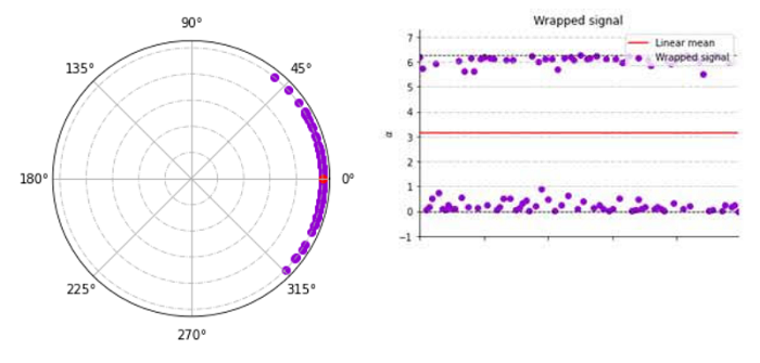
Conventional methods suitable for the analysis of linear data don’t fit angular data. First, let’s consider a zero-mean – normally distributed angular signal with standard deviation (std) of 0.3 radian.  At first glance, when examining this distribution over the real plane (Fig 1.a), it appears to come from two populations being wrapped between 0 to 2π rad. Calculating the familiar linear arithmetic mean will return π as a result, but, after the signal is represented as points on the circumference of a unit circle (Fig 1.b), it is clear that the mean is actually 0 rad.

By assuming linearity, we ignore the data’s real topography: any two points 2π apart in the real plane will be transformed into the same location over the unit circle. Disregarding the periodic nature of the signal makes many linear techniques often misleading.

So, what can we do?

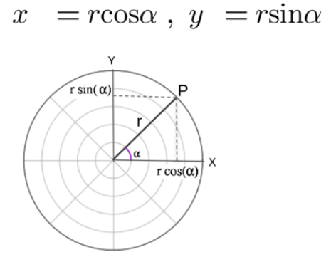
By using polar transformation, we can map the distribution to Cartesian coordinates. Any point over the circle can be described as (X,Y) in terms of Cartesian coordinates, using the trigonometric functions cosine and sine for the translation:

Wher e is an angle in [0, 2π) and r set to a const value of unit length
(r = 1) for convenience.

Algorithm:

1. Convert each sample to 2d representation from polar coordinates to Cartesian coordinates.
2. Calculate the arithmetic mean over each component separately.

3. Convert back using atan2.

Code:

Circular Median

In order to compute the median of circular data, we must first address the question of ‘circular distance’ – the difference in the measured values of two points when the data that they represent is angular.

How Do We Estimate The Circular Distance?

The most popular measure for distance is the Euclidean distance, which works perfectly on linear data in the Euclidean space. In the “circular world”, there are a couple of strong candidates when the most intuitive among them is based on arc lengths, taking the smaller of the two arc-lengths between the points along the circumference:

Where  and  represent the angles corresponding to the points A, B over the unit circle. The red arc is shorter than the purple, hence, we define the circular distance to be the arclength ACB. The circular distance always lies in [0,π) since there are no two points on the circumference of a circle that can be farther than π.

Code:

Let’s use the definition of “circular distance” for calculating the median of a distribution.

In statistics, a median is a value separating the higher half from the lower half of a data sample. It can be handy when treating non-Normal distributions because it is less affected by a small proportion of extremely large or small values. The median of a data sample can be defined as the observation with the minimum distance to all the other observation in the sample. What’s left is to combine the definition of the median with the definition of circular distance:

Where d is the circular distance between two angular observations.

Code:

Removing undesirable aspects of a signal is always very important, as it will reduce noise and improve the data quality for better modeling and data inference. Analyzing circular data is tricky, however, analyzing noisy circular data might prove to be quite challenging.

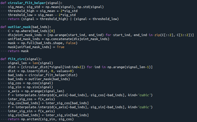
We discussed the polar transformation and reviewed powerful tools for analysis: mean, median and “circular distance”. Now if we combine these to construct our filter through the following steps:

1. Calculate the distance between two adjacent samples.
2. Set low and high thresholds for this distance.
3. Filter the observation above or below these thresholds.
4. Convert each sample to Cartesian coordinates.
5. Use a ‘cubic’ interpolation on each component separately.
6. Recombine using atan2.

We will have this code:

Ultimately, there are big differences between linear and circular data, which is why it is so important to use the appropriate techniques and models for such data. By also using algorithms for calculating mean and distance and by filter outliers, these are the first steps one can take in exploring the world of directional data.

About the Author

Amit Babayoff is a data scientist at Deeyook, a precise location technology company that develops indoor and outdoor navigation solutions. Amit holds a Master’s Degree in Computation Neuroscience and a Bachelor’s Degree in CS and Neuroscience .She has a strong interest in ML, (biological and computer) vision and robotics, and enjoys solving complicated problems in multidisciplinary fields.

Sign up for the free insideAI News newsletter.

Join us on Twitter: @InsideBigData1 – https://twitter.com/InsideBigData1